Electrochemistry

Introduction to Electrochemistry

Electrochemistry is the study of interchange of chemical and electrical energy.

Oxidation/Reduction involves the exchange of electrons from one chemical species to another. Normally, this is done when the two chemicals contact each other in the activated complex (when two species bump into each other in solution for example).

We are interested in separating the chemical species such that the electrons transfer via an external circuit. That way, we can measure the electrochemical effects.

To properly understand the connection between the redox reaction and the electricity, we should balance the overall redox reaction using a half-reaction method such as the one described in the previous section of these notes. We can set up the physical reaction vessel such that the chemicals from one half reaction are separated from those of the second half reaction. For reaction to occur, we still need to connect the solutions to complete the circuit. This is done by attaching wires between electrodes in the two half cells and by connecting the solutions of the two half cells via a salt bridge or by some other device such as a semi-permeable membrane.

In general, such a cell is called an electrochemical cell. These cells could be used in one of two types of situations:

1. The chemical reaction is spontaneous and produces electricity.
   This is called a voltaic cell or a galvanic cell.
2. The chemical reaction is non-spontaneous and is forced by electricity from an external source.
   This kind of cell is called an electrolysis cell.

We will look at the first situation first.

Galvanic or Voltaic cells

Consider a piece of zinc foil placed in a beaker of copper sulphate. The copper sulphate solution is blue because of the presence of the Cu²⁺ ions. When the zinc is added, the solution changes to colourless and the zinc metal is dissolved and replaced by a reddish orange powder. The colourless solution no longer has Cu²⁺ in it and the reddish orange powder is Cu(s). The Zn(s) is dissolved and is now Zn²⁺. [I know this because of my vast knowledge of chemistry ;-)]

If we write an overall reaction for this process, we get:

Zn + Cu²⁺  Zn²⁺ + Cu. This doesn't help us in our quest for electrochemistry knowledge. Let's rewrite this in half-reaction form.

Zn  Zn²⁺ + 2e^-

Cu²⁺ + 2e^-  Cu

Now, we can set up two half cells, one with a zinc electrode in a Zn²⁺ solution (say ZnSO₄) and the other with a copper electrode in a Cu²⁺ solution (say CuSO₄) as follows.

The centre line in the diagram, recall, is either a semi-permeable membrane or a salt bridge.

Now, at the anode, we have the reaction

Zn(s)  Zn²⁺(aq) + 2e^-(aq)

and at the cathode, we have

Cu²⁺(aq) + 2e^-(aq)  Cu(s)

Electrons pass through the wires and SO₄^2- pass through the membrane to keep the solutions neutral.

Cell Potentials

Electrons from solution pushed onto the anode, around the external circuit and onto the cathode where they are pulled out into the solution.

That's one way of thinking of the electrical circuit part of the electrochemical cell. The electrons pushed around the external circuit can do work (run a motor, illuminate a light bulb, etc). The amount of work possible is a function of both the voltage (potential) and of the current (number of electrons) in the circuit.

Pushing one Coulomb of charge around a circuit at a potential of 1 Volt does One Joule of work. OR, mathematically, 1J = 1V × 1C.

The cell potential (voltage of the cell) depends on the chemicals used. For example, the chemicals in dry-cells(batteries) are such that the potential is always about 1.5 V. This has become a standard and is now a limiting factor in deciding which chemicals can be used to create a battery.

The cell potential is given a symbol of E_cell. If all chemicals are at activity of 1 (conc. = 1 M, p = 1 bar) then the cell potential is the standard cell potential and is given as E°_cell.

Any redox reaction has the potential (pun) to be used in an electrochemical cell. We merely need to be able to divide the oxidizing and reducing agents into two half cells (half reactions).

Take for example, the reaction of zinc metal dissolving in hydrochloric acid. The reaction is:

Zn(s) + 2H⁺(aq)  Zn²⁺(aq) + H₂(g)

We need to separate the zinc from the hydrogen. We can use zinc as an electrode but what about the hydrogen.

In this case, we need to set up a special electrode, which allows H₂ gas molecules to interact directly with H⁺dissolved in water and with the electrons from the external circuit simultaneously. Such a system is pictured below.

A blow-up of the surface of the platinum electrode is shown below so the location of reaction can be better understood.

The other half-cell would look much like that pictured in a previous diagram. The whole cell diagram, of course would include the external part of the circuit and the salt bridge or membrane to complete the circuit. We can abbreviate this diagram as follows:

Zn(s)/ZnSO₄(aq)//H₂SO₄(aq)/H₂(g),Pt(s)

  [Anode             //            Cathode]

Where the single slash mark / represents the boundary between solution and electrode and the double slash //represents the salt bridge or semi-permeable membrane. The external circuit, of course, joins the two electrodes (solid) and is not explicitly shown here.

The overall cell voltage can be summed from the half-cell potentials of the oxidation and of the reduction reactions.

E_cell = E_Red + E_ox.

Standard Reduction Potentials

As before, we wish to tabulate thermodynamic data in some useable way. We define a standard set of conditions under which all half-reactions can theoretically operate and we tabulate the half-cell potentials for the reactions under standard conditions. Since the potential of an oxidation reaction (loose electron) is merely the negative of the potential for a reduction reaction reaction (gain electron), we choose to tabulate only the reduction half-reactions. Any oxidation half reactions are merely the reverse of the tabulated reduction reaction and the oxidation potential is the negative of the tabulate reduction potential.

Table D.4 from Petrucci lists many reduction half-reactions that you will need for problems, etc in the text.  Herein, I have duplicated only a few in the following table.

	reduction	Eº/volts
1	O2 + 4H+ + 4e-  2H2O	+1.229
2	Ag+ + e-  Ag	+0.7996
3	Cu2+ + 2 e-  Cu	+0.3419
4	Fe2+ + 2 e-  Fe	-0.447
5	Zn2+ + 2 e-  Zn	-0.7628
6	2H2O + 2e-  H2 + 2OH-	-0.83
7	Na+ + e-  Na	-2.71

A few years ago, a city experienced a number of very serious water main breaks on sections of pipe that had been recently replaced. The City engineer was fired. His onlydefence was "How was I to know that brass fittings (mostly copper) on cast iron pipes would corrode so fast." Was the city justified in firing him? Can you explain their reasoning for calling him incompetent?

Let's look at this small reduction potential table and see if we can use it to explain certain experimentally observable properties of matter.  First off, I should point out that the more positive reduction potentials refer to more spontaneous reduction reactions.

The first reaction in this mini-table shows the reduction of oxygen. This is higher in the table than many other things. That makes sense since we know that oxygen is a good oxidizing agent (it makes other things oxidize while it itself is reduced).

We can see that water can be both oxidized (-1) and reduced (2). It is oxidized to oxygen and reduced to hydrogen. These two reactions, in fact, serve as a set of boundaries for aqueous solutions. Any materials harder to oxidize than water will not oxidize since the water will.  Similarly, any materials harder to reduce than water will never reduce (in water). For example, sodium ions will never reduce to sodium metal in the presence of water since the water will reduce first.  In fact, sodium metal in water will spontaneously (explosively) oxidize to Na⁺ ions and the water will reduce to hydrogen gas and leave a basic solution (equation 6). The overall reaction for this process is the sum  (#6) - 2×(#7).

NOTE: when we add half-cells, their potentials are strictly additive.  We don't multiply or divide by any factors even though we do so to the stoichiometric coefficients of the equations in order to balance the overall equation.  Potentials don't depend on the total amount or size of the cell, just the concentrations.  You already know this.  If you buy a AA cell or a D cell, their voltages are both 1.5V. However, their capacity to do work is not the same.

2Na + 2 H₂O  2Na⁺ + H₂ + 2OH^-

Thus, the overall standard cell potential for this reaction is

Eº_cell = Eº_red + Eº_ox = -0.83 + 2.71 (reverse reaction => change sign) = 1.88 V.

Positive cell potential means spontaneous reaction.

When pairing up metals, we know that zinc will dissolve in a copper (II) solution. Here we see that the copper (II) (3) is easier to reduce than the zinc (II) (5)

18-Electron rule

The 18-electron rule is a rule used primarily for predicting formulae for stable metal complexes.The rule is based on the fact that the valence shells of transition metals consist of nine valence orbitals, which collectively can accommodate 18 electrons as either bonding or nonbonding electron pairs. This means that, the combination of these nine atomic orbitals with ligand orbitals creates nine molecular orbitals that are either metal-ligand bonding or non-bonding. When a metal complex has 18 valence electrons, it is said to have achieved the same electron configuration as the noble gas in the period. The rule and its exceptions are similar to the application of the octet rule to main group elements. The rule is not helpful for complexes of metals that are not transition metals, and in fact the majority of transition metal complexes violate the rule. The rule was first proposed by American chemist Irving Langmuir in 1921.

Applicability of the 18-electron rule

Although the majority of metal complexes do not satisfy the 18-electron rule, the rule usefully predicts the formulae for low-spin complexes of the Cr, Mn, Fe, and Co triads. Well-known examples include ferrocene, iron pentacarbonyl, chromium carbonyl, and nickel carbonyl.
Ligands in a complex determine the applicability of the 18-electron rule. In general, complexes that obey the rule are composed at least partly of π-acid ligands. This kind of ligand exerts a very strong ligand field, which lowers the energies of the resultant molecular orbitals and thus favorably occupied. Typical ligands include olefins, phosphines, and CO. Complexes of π-acids typically feature metal in a low-oxidation state. The relationship between oxidation state and the nature of the ligands is rationalized within the framework of π backbonding.

Consequences for reactivity

Compounds that obey the 18 VE rule are typically "exchange inert." Examples include [Co(NH₃)₅Cl]²⁺, Mo(CO)₆, and [Fe(CN)₆]^4-. In such cases, in general ligand exchange occurs via dissociative substitution mechanisms, wherein the rate of reaction is determined by the rate of dissociation of a ligand. On the other hand, 18-electron compounds can be highly reactive toward electrophiles such as protons, and such reactions are associative in mechanism, being acid-base reactions.
Complexes with fewer than 18 valence electrons tend to show enhanced reactivity. Thus, the 18-electron rule is often a recipe for non-reactivity in either a stoichiometric or a catalytic sense.

Alternative analysis

In the prevalent LF analysis, the valence p orbitals on the metal participate in metal-ligand bonding, albeit weakly. Some new theoretical treatments do not count the metal p-orbitals in metal-ligand bonding, although these orbitals are still included as polarization functions. This results in a dodectet (12) rule which accommodates all low-spin complexes including linear 14e complexes such as Tollen's reagent and square planar 16e complexes as well as implies that such transition metal complexes are hypervalent, but has yet to be adopted by the general chemistry community.

Exceptions to the 18-electron rule

π-donor or σ-donor ligands with small interactions with the metal orbitals lead to a weak ligand field which increases the energies of t_2g orbitals. These molecular orbitals become non-bonding or weakly anti-bonding orbitals (small Δ_oct). Therefore, addition or removal of electron has little effect on complex stability. In this case, there is no restriction on the number of d-electrons and complexes with 12 -22 electrons are possible. Small Δ_oct makes filling e_g* possible ( > 18e-) and π-donor ligands can make t_2g antibonding ( < 18 e-). These types of ligand are located in low to medium of the spectrochemical series. For example: [TiF₆]^2- (Ti⁴⁺, d⁰, 12 e), [Co(NH₃)₆]³⁺ (Co³⁺, d⁶, 18 e), [Cu(OH₂)₆]²⁺ (Cu²⁺, d⁹, 21 e) In tems of metal ions, Δ_oct increases down a group as well as increasing oxidation number. Strong ligand fields lead to low-spin complexes which cause some exceptions to 18-electron rule.

16e complexes

A popular class of complexes that violate the 18e rule are the 16e complexes with d⁸ configurations. All high-spin d⁸metal ions are octahedral (or tetrahedral), but the low-spin d⁸ metal ions are all square planar (Jahn-Teller distortion). Important examples of square-planar low-spin d⁸ metal Ions are Ni(II), Pd(II), and Pt(II). At picture below is shown the splitting of the d sub-shell in low-spin square-planar complexes. Examples are especially prevalent for derivatives of the cobalt and nickel triads. Such compounds are typically square-planar. The most famous example is Vaska's complex (IrCl(CO)(PPh₃)₂), [PtCl₄]²⁻, and Zeise's salt [PtCl₃(η²-C₂H₄)]⁻. In such complexes, the d_z2 orbital is doubly occupied and nonbonding.

Many catalytic cycles operate via complexes that alternate between 18e and square-planar 16 configurations. Examples include Monsanto acetic acid synthesis, hydrogenations, hydroformylations, olefin isomerizations, and some alkene polymerizations.
Other violations can be classified according to the kinds of ligands on the metal center.

Bulky ligands

Bulky ligands can preclude the approach of the full complement of ligands that would allow the metal to achieve the 18 electron configuration. Examples:

• Ti(neopentyl)₄ (8 VE)
• Cp*₂Ti(C₂H₄) (16 VE)
• V(CO)₆ (17 VE)
• Cp*Cr(CO)₃ (17 VE)
• Pt(P^tBu₃)₂ (14 VE)
• Co(norbornyl)₄ (13 VE)
• [FeCp₂]⁺ (17 VE)

Sometimes such complexes engage in agostic interactions with the hydrocarbon framework of the bulky ligand. For example:

• W(CO)₃[P(C₆H₁₁)₃]₂ has 16 VE but has a short bonding contact between one C-H bond and the W center.
• Cp(PMe₃)V(CHCMe₃) (14 VE, diamagnetic) has a short V-H bond with the 'alkylidene-H', so the description of the compound is somewhere between Cp(PMe₃)V(CHCMe₃) and Cp(PMe₃)V(H)(CCMe₃).

High-spin complexes

High-spin metal complexes have singly occupied orbitals and may not have any empty orbitals into which ligands could donate electron density. In general, there are few or no π-acidic ligands in the complex. These singly occupied orbitals can combine with the singly occupied orbitals of radical ligands (e.g., oxygen), or addition of a strong field ligand can cause electron-pairing, thus creating a vacant orbital that it can donate into. Examples:

• CrCl₃(THF)₃ (15 VE)
• [Mn(H₂O)₆]²⁺ (17 VE)
• [Cu(H₂O)₆]²⁺ (21 VE, see comments below)

Complexes containing strongly pi-donating ligands often violate the 18-electron rule. These ligands include fluoride (F⁻), oxide (O²⁻), nitride (N³⁻), alkoxide (RO⁻), and imide (oxide (RN²⁻). Examples:

• [CrO₄]²⁻ (16 VE)
• Mo(=NR)₂Cl₂ (12 VE)

In the latter case, there is substantial donation of the nitrogen lone pairs to the Mo (so the compound could also be described as a 16 VE compound). This can be seen from the short Mo-N bond length, and from the angle Mo - N - C(R), which is nearly 180°. Counter-examples:

• trans-WO₂(Me₂PCH₂CH₂PMe₂)₂ (18 VE)
• Cp*ReO₃ (18 VE)

In these cases, the M=O bonds are "pure" double bonds (i.e., no donation of the lone pairs of the oxygen to the metal), as reflected in the relatively long bond distances.

Pi-donating ligands

Ligands where the coordinating atom bear nonbonding lone pairs often stabilize unsaturated complexes. Metal amides and alkoxides often violate the 18e rule.

Combinations of effects

The above factors can sometimes combine. Examples include

• Cp*VOCl₂ (14 VE)
• TiCl₄ (8 VE)

Higher electron counts

Some complexes have more than 18 electrons. Examples:

• Cobaltocene (19 VE)
• Nickelocene (20 VE)
• The hexaaqua copper(II) ion [Cu(H₂O)₆]²⁺ (21 VE)

Often, cases where complexes have more than 18 valence electrons are attributed to electrostatic forces - the metal attracts ligands to itself to try to counterbalance its positive charge, and the number of electrons it ends up with is unimportant. In the case of the metallocenes, the chelating nature of the cyclopentadienyl ligand stabilizes its bonding to the metal. Somewhat satisfying are the two following observations: (i) cobaltocene is a strong electron donor, readily forming the 18-electron cobaltocenium cation and (ii) nickelocene tends to react with substrates to give 18-electron complexes, e.g. CpNiCl(PR₃) and free CpH.

Atomic and Molecular spectroscopy

Atomic Spectroscopy

Atomic spectroscopy exploits different energetic transitions experienced by atoms that are associated with either the absorption or emission of photons. When these transitions involve the excitation and relaxation of the valence (outer or bonding) shell electrons of metal atoms and ions, the corresonding photons have energies within the ultraviolet and visible regions of the spectrum. A good example of this is the dark absorption lines in the solar spectrum, which are caused by heavier elements present in the outer layers of the sun.

The figure on the right shows a high energy photon with Ephoton = hν being absorbed, resulting in a 2s→3s electron excitation; similarly, a 3d→3p electron relaxation results in the emission of a lower energy photon. By convention, the change in electron energy ΔE = Ef − Ei, where f and i refer to the final and initial states, respectively; so ΔE =Ephoton, and the sign of Ephoton tells you whether the photon is being absorbed or emitted. Since Ef and Ei depend on the number electrons and protons within an atom (or monatomic ion), the wavelengths associated with atomic absorption and emission are considered characteristic for a particular element.

Absorption and Emission:

In atomic absorption (AA) spectroscopy, absorption of a photon results in excitation of an electron from a lower to higher energy atomic orbital (AO). An instrument measures the absorbance, A, which is defined as the logarithm of the ratio of incident to transmitted radiant power of the photon beam, A = log(P0 ÷ P), at a wavelength specific to the element of interest. Samples are typically analysed using a flame atomic absorption spectrophotometer.

In atomic emission (AE) spectroscopy, thermal or electrical energy from an arc, flame, spark, or plasma is used to excite and electron from a lower to higher energy AO; when the excited electron returns to its original AO (i.e. the ground state), it may do so by emitting a photon. The instrument measures the intensity,I, of these emitted photons as a function of wavelength.

Because AO energies are well-defined, atomic absorption and emission spectra consist of discrete, narrow lines. This allows the concentration of metallic elements in different samples to be determined selectively, with lower limits at or below 1 mg/L (1 ppm). Techniques such as graphite furnace atomic absorption spectrophotometry (GFAAS) allow concentration to be measured down to µg/L (ppb) levels. Actual limits-of-detection vary with both element, technique, and sample matrix.

Molecular Spectroscopy

Introduction

Spectroscopy is the use of the absorption, emission, or scattering of electromagnetic radiation by atoms or molecules (or atomic or molecular ions) to qualitatively or quantitatively study the atoms or molecules, or to study physical processes. The interaction of radiation with matter can cause redirection of the radiation and/or transitions between the energy levels of the atoms or molecules. A transition from a lower level to a higher level with transfer of energy from the radiation field to the atom or molecule is called absorption. A transition from a higher level to a lower level is called emission if energy is transfered to the radiation field, or nonradiative decay if no radiation is emitted. Redirection of light due to its interaction with matter is called scattering, and may or may not occur with transfer of energy, i.e., the scattered radiation has a slightly different or the same wavelength.

Absorption

When atoms or molecules absorb light, the incoming energy excites a quantized structure to a higher energy level. The type of excitation depends on the wavelength of the light. Electrons are promoted to higher orbitals by ultraviolet or visible light, vibrations are excited by infrared light, and rotations are excited by microwaves.
An absorption spectrum is the absorption of light as a function of wavelength. The spectrum of an atom or molecule depends on its energy level structure, and absorption spectra are useful for identifying of compounds.
Measuring the concentration of an absorbing species in a sample is accomplished by applying the Beer-Lambert Law.

Emission

Atoms or molecules that are excited to high energy levels can decay to lower levels by emitting radiation (emission or luminescence). For atoms excited by a high-temperature energy source this light emission is commonly called atomic or optical emission, and for atoms excited with light it is called atomic fluorescence. For molecules it is called fluorescence if the transition is between states of the same spin and phosphorescence if the transition occurs between states of different spin.
The emission intensity of an emitting substance is linearly proportional to analyte concentration at low concentrations, and is useful for quantitating emitting species.

Scattering

When electromagnetic radiation passes through matter, most of the radiation continues in its original direction but a small fraction is scattered in other directions. Light that is scattered at the same wavelength as the incoming light is called Rayleigh scattering. Light that is scattered in transparent solids due to vibrations (phonons) is called Brillouin scattering. Brillouin scattering is typically shifted by 0.1 to 1 cm^-1 from the incident light. Light that is scattered due to vibrations in molecules or optical phonons in solids is called Raman scattering. Raman scattered light is shifted by as much as 4000 cm^-1 from the incident light.

Structure and bonding of Metalic carbonyls

we will here study the structure and bonding of ...:

i) Mononuclear carbonyls:-

The structure of mononuclear metalic carbonyls have been studied by x-ray difraction, IR spectroscopy and electron difraction. All the mononuclear carbonyls have linear metal-carbonyl bond in which metal atom is linked to carbonyl molecule through the carbon atom since oxygen atom is more electronegative than carbon atom.

Sapes of metal carbonyls:-

i) Hexacarbonyls:-

                           The carbonyls having six carbonyl molecules attached to metal atom are called hexacarbonyls.

                           Shape = Octahedral

                           Hybridization = d2sp3

                          Co-ordination number = 6

Examples:-

               V ( CO)6, Cr(CO)6, W(CO)6

ii) Pentacarbonyls:-

                              Such carbonyls ehich contain five carbonyl molecules attached to the metal atom are called pentacarbonyls.

                         Shape = Trigonal bipyramidal

                         Hybridization = dSp3

                         Co-ordination number = 5

Examples:-

               Fe(CO)5, Ru(CO)5, Os(CO)5

iii) Tetracarbonyls:-

                               The carbonyls which contain four carbonyl molecules attached o the metal atom are called tetracarbonyls.

                           Shape = tetrahedral / Square planner

                   Hybridization= Sp3         / dSp2

                     Co-ordination number = 4

Example:-

                Ni(CO)4

Metal carbonyl

Metal carbonyls are coordination complexes of transition metals with carbon monoxide ligands. They occur as neutral complexes, as positively charged metal carbonyl cations or as negatively charged metal carbonylates. The carbon monoxide ligand may be bound terminally to a single metal atom or bridging to two or more metal atoms. These complexes may be homoleptic, that is containing only CO ligands, such as nickel carbonyl (Ni(CO)₄), but more commonly metal carbonyls are heteroleptic and contain a mixture of ligands.

Metal carbonyls are useful in organic synthesis and as catalysts or catalyst precursors in homogeneous catalysis, such as hydroformylation and Reppe chemistry. In the Mond process, nickel carbonyl is used to produce pure nickel. In organometallic chemistry, metal carbonyls serve as precursors for the preparation of other organometalic complexes.

Metal carbonyls are toxic by skin contact, inhalation or ingestion, in part because of their ability to carbonylate hemoglobin to give carboxyhemoglobin, which prevents the binding of O₂.

In metalic carbonyls, metals are in zero oxidation state.

Metal carbonyls of transition elements constitute another important class of organometallic compounds. All d-block elements which contain only carbonyl ligands are called homoleptic carbonyls.

Amond in 1890 prepared the first homoleptic carbonyl, Ni(CO)₄. Later on a large number of neutral binary carbonyl like, Fe(CO)₅, Cr(CO)₆, Mo(CO)₆, W(CO)₆ were prepared. In addition to mononuclear metal carbonyls mentioned above, transition metals from many polynuclear metal carbonyls such as Fe₃(CO)₁₂, Mn₂(CO)₁₀. The metal carbon bonds in metal carbonyls possess both σ and π character.

Classification of metal carbonyls

Metal carbonyls are classified into two types:

(i) Mononuclear (or monomeric) carbonyls: these are such compounds which contain only one metallic atom per molecule. For example, V(CO)₆, Cr(CO)₆, etc.

(ii) Polynuclear carbonyls: these contain two or more metallic atoms per molecule and are of the type M_x(CO)_y. These carbonyls are also sometimes called as bridged carbonyls. Polynuclear carbonyls may be homonuclear e.g., Fe₃(CO)₁₂ or heteronuclear e.g.,MnCo(CO)₉, MnRe(CO)₁₀.

Nomenclature of metal carbonyls

(i) In metal carbonyls the metal atom is in zero oxidation sate therefore it may not be mentioned.

(ii) If the metal atom appears two or more times than the word di, ter etc is added before the name of metal atom.

(iii) If the CO groups act as bridge between the two metals atoms then the Greek letter mu () is written before their names.

(iv) When the metal-metal bond is present between similar atoms than the multiple prefixes, bis, tris, etc. are taken.

(v) While writing the names of π bonded organometallic compounds the symbol prefixes, hapto (η) is used before the name of molecule indicating the number of carbon atoms in the carbon bonded ligand.

Some examples are given below to illustrate the above points.
                                           
Ni(CO)₄ Tetracarbonylnickel
                                 
Mn₂(CO)₁₀ decacarbonyl dimanganese
                                     
Co₂(CO)₈ Octacarbonyl dicobalt
                                      
Fe(CO)₉ Enneacarbonyldiiron
                      
(CO)₃-Co-(CO)₂-Co(CO)₃ Di--carbonyl bis (tricarbonyl cobalt)
                           
(CO)₄Co-Co-(CO)₄ Bis (tetracarbonyl cobalt)
                          
(CO)₃Fe(CO)₃Fe(CO)₃ Tri--Carbonyl bis (tricarbonyl iron)
                         
(C₆H₆) Cr(CO)₃ (η₆-benzene) tricarbonyl chromium   
                         
Fe(CO₃) (C₄H₆) (η₄-butadiene) tricarbonyl iron.

Bonding in metal carbonyl

As already mentioned, the M-C bond in metal carbonyls has σ as well as π character. The metal-carbon σ bond is formed by the donation of lone pair of electrons on the carbonyl carbon into a vacant orbital of the metal. The metal-carbon π bond is formed by the donation of a pair of electrons from a filled d-orbital of metal into the vacant antibonding pi-molecular orbital (π) of carbon monoxide.

The metal to ligand bonding generates a synergic effect that reinforces the bond between CO and the metal.

Preparation of metal carbonyls

Finely divided nickel reacts with CO at room temperature to form Ni(CO)₄.
                                                 
Ni + 4CO    Ni(CO)₄

Iron reacts with CO at higher temperature and pressure.
                                                 
Fe + 5CO    Fe(CO)₅

Nickel can be purified by first converting it into volatile Ni(CO)₄ and subsequent thermal decomposition of Ni(CO)₄. This process is known as Mond process.

Properties of metal carbonyls

1. Metal carbonyls are generally solids at room temperature and pressure. However Nickel carbonyls are liquids.

2. The mononuclear carbonyls are unstable and noxious.

3. Mononuclear carbonyls are either colourless or light coloured whereas polynuclear carbonyls are more deeply coloured. For example, Fe(CO)₅ is light straw coloured liquid while Fe₃(CO)₁₂ is a deep green solid.

4. With exception of Fe2(CO)₉, carbonyls are soluble in hydrocarbon solvents.

Examples of Spectroscopy in Astronomy

Spectroscopy is a powerful tool in astronomy -- from it, we can often get information about the temperature, density, composition, and important physical processes of an astronomical object. This information can help us answer the questions:

• What is it?
• What is it like?
• What is it made out of?
• How did it get there? What will happen to it?
• Does it give us clues as to how WE got here?

A few examples of astronomical spectra are highlighted here. Some cool Astronomy Camp spectra also live in these pages.

---

Molecular Spectroscopy and Comets

Comets consist of almost pristine material from the early formation of our solar system, unprocessed by harsh solar sunlight. Studying the chemistry of these "dirty snowballs" gives us a clue as to the composition and nature of our solar system in its infancy and constrains theories of how life may have formed on Earth.
A link to radio-wavelength spectroscopy of comets may be found here.

---

Probing the Formation of Stars in Colliding Galaxies

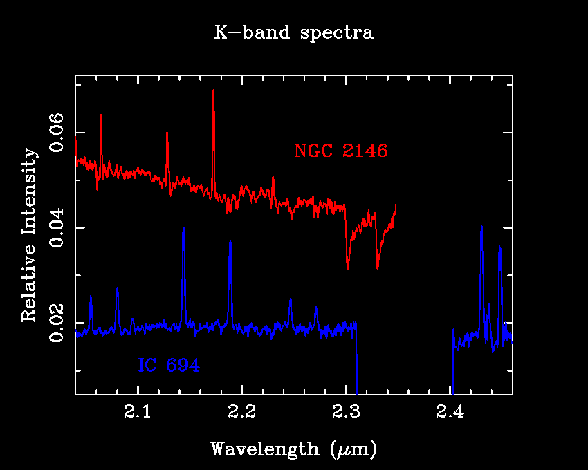
Billions of years ago, when our galaxy took form, it is thought that there must have been an epoch of rapid star-forming activity that has since subsided. We can get clues to how this may have looked by observing galaxies currently exhibiting violent, extreme star-formation. Such "starburst" galaxies are studied best in the infrared and at radio wavelengths, since star-forming galaxies often harbor so much dust and gas that visible light cannot penetrate to the centers where the majority of the star formation is taking place. Below is an infrared (2.0 - 2.5 microns wavelength, or 20,000 - 25,000 Angstroms) spectrum of two such starburst galaxies. Most of the features you see are from molecular hydrogen, H₂, the stuff from which stars are made! These molecular hydrogen emission lines tell us that the molecular gas we see is very warm; in the top galaxy, the gas is excited by shock-heated gas. The bottom galaxy has molecular hydrogen excited by ultraviolet light emitted from recently-formed young, hot stars.

---

Uncovering the mystery of Quasars

The distant nature of quasars were discovered in the early 1960's, when spectral lines were noted to be substantially-shifted redder than they should normally be. This redshift can be attributed to the recession (speeding away) of quasars from us. In the standard Big Bang model of cosmology (the faster it's speeding away from you, the more distant it is), this rapid motion implies that quasars are the most distant objects known. Below is a typical spectrum of a quasar. The wavelength scale has been rescaled to the "appropriate" rest wavelengths for the spectral lines. The most noticeable feature is the broad emission line at 1216 Angstroms due to hydrogen atoms making the transition from the first excited state to the ground state. Although 1216 Angstroms lies deep in the ultraviolet, where the Earth's atmosphere is opaque, many quasars are receding from us so fast, this line is redshifted into the visible part of the spectrum (4000-7000 Angstroms).

Spectroscopy at Astronomy Camp!

Spectroscopy at Astronomy Camp is done with a spectrograph from Optomechanics Research Inc, coupled with the Mount Lemmon 40" or 60" telescopes and the Camp's SBIG ST6 CCD detector array. With relatively short exposure times, good quality spectra can be taken of most catalogued stars and high surface-brightness deep-sky objects. A few examples of Astronomy Campers' handiwork are shown below.

Planetary Nebulae, Or 'Why Light Pollution Filters Work'!

Here's an image of M57 (a.k.a. the Ring Nebula), with a crude representation of the spectrometer slit superimposed. This image is a 180 second exposure using the Camp's ST6 CCD on a 10" Meade Schmidt-Cassagrain telescope. Astronomy Camp's spectrograph was mounted on the Mount Lemmon 60" telescope with the same ST6 CCD. The slit length is about 8 arcminutes long and 1 arcsecond wide; the representation of the slit width in the diagram is exaggerated.

We combined four 5-minute exposures on the Ring Nebula using the 60" and the ST6 camera. We subtracted an appropriate 5 minute dark frame from each image and then combined the images using IRAF. The resulting ST6 image follows: the dispersion (wavelength) axis is horizontal, and the spatial axis (along the Ring Nebula) is vertical. The central lines are M57, the upper and lower spikes are the calibration lamp spectra (Hg+He).

We make a 1-D spectrum from the 2-D image by summing over the aperture of the slit covering M57. Using the well-characterized wavelengths of the calibration lamps, we can use IRAF to register our spectrum to provide a nice wavelength scale. Here's what our spectrum looks like once plotted as intensity versus wavelength.

The emission line at 4861 Angstroms comes from hot, excited atomic hydrogen. Highly-excited hydrogen atoms in M57's gaseous shell, starting in energy level 4, may eventually de-excite to level 2, giving up the energy difference in waves of light at that particular energy (and... they have a wavelength of 4861 Angstroms!).

The brightest two lines at 4959 and 5007 Angstroms come from twice-ionized oxygen (labeled O++, or O III in spectroscopic notation). This means that two of oxygen's eight electrons have been ripped away. This is a also clue that conditions in this nebula must be harsh. In fact, these lines can only be excited to emit light in temperatures of several thousand Kelvins and rather thin densities of 1-100 atoms per cubic centimeter. There is no continuous spectrum here -- this points out the important fact that planetary nebulae are hot rarified gases -- you see a LINE spectrum. This also points out how astronomers can get valuable information about the physical conditions and important processes in distant astronomical objects.
This spectrum also demonstrates why you can use light-pollution filters (like those made by Lumicon or Orion) to get great contrast from reflection/emission nebulae! These filters pass light waves that lie at wavelengths covered by these three lines, but block light at all other wavelengths. For nebulae, this is very beneficial since they only emit visible light in this wavelength range. You can remove all that ugly skyglow and light pollution without reducing the brighness of the nebula you're looking for.
Would such a narrow-band filter be good for looking at stars or galaxies? Hmm?

---

Stellar Spectroscopy

A look at Sirius Now, onto stellar spectroscopy. This 1/2 second exposure of Sirius is centered near 4000 Angstroms (blue, near-ultraviolet) and clearly shows a series of deep absorption lines. These lines are due to the hydrogen atom. Let's explore how.
In the cooler outer "atmosphere" around Sirius, mildly excited hydrogen atoms in the 2nd energy level (the 1st excited state) are 'zapped' by photons (light waves) with just the right energy to send them to even higher excited states. In this figure, we match the dark absorption line that results from each transition upward in the hydrogen atom. Notice that the higher-energy transitions on the left result in higher energy absorption lines out in the ultraviolet. This series of lines, starting from level 2, is called the Balmer series after their discoverer.
Stars are classified by their temperatures, which can be determined by the star's spectral features. The hottest stars are termed O-stars, the next cooler are B stars, then A, F, G, K, and finally M-stars. Sirius is a relatively hot A-type star at about 10,000 degrees Kelvin. Such stars have the strongest hydrogen-features (simply due to temperature -- cooler stars can't 'zap' the hydrogen atoms as effectively, and hotter stars will destroy/ionize the hydrogen atoms that create the spectral lines!).

---

Molecules in Cool Stars! On the other end of the scale -- here is Delta Virgo; a cool M3-type giant star at about 3,500 K and viewed at about 6000 Angstroms (in red light). Note a bright continuum at far left, which suddenly dims into a series of striations (bands). These don't look like the sharp absorption lines of the hydrogen atom, do they? In fact, these bands are due to MOLECULES that can live in the atmospheres of these cool stars! This particular molecule is TiO (titanium oxide). Molecules have a dizzying number of lines because they not only have the electron energy levels like atoms, but also have energy sublevels due to the rotation and vibration of the molecule! At the modest resolution of our spectrometer, these hundreds of lines are blended into absorption bands like what we see here.

---

Stars like our Sun Somewhere between hotter A-type stars and cool M-class stars are stars like our sun, around 5500 degrees Kelvin. Here's Beta-Bootes, a G8 giant star (roughly what our sun will be when it begins dying in about 5 billion years). The first spectrum is at 5500 Angstroms (yellow light), just like the M-star spectrum above. Notice that molecules don't form here (it's too hot for molecules to readily form without being quickly destroyed), but there are still an awful lot of lines around. Most of these features are due to heavy elements -- things like carbon (in several ionization stages), iron, oxygen, magnesium, calcium etc.

This is a spectrum of the same star, but now taken at 4000 Angstroms (deep blue-violet light). The deep absorption lines at left are due to the ion Calcium II (the difference between this and normal, neutral calcium is that one electron has been stripped off here). The small dip in the middle is due to a blend of metallic features and hydrogen. Notice that the hydrogen lines are very weak here -- nothing at all like Sirius (a hotter A-class star).

Spectroscopy

What is Spectroscopy? Spectroscopy pertains to the dispersion of an object's light into its component colors (i.e. energies). By performing this dissection and analysis of an object's light, astronomers can infer the physical properties of that object (such as temperature, mass, luminosity and composition).
But before we hurtle headlong into the wild and woolly field of spectroscopy, we need to try to answer some seemingly simple questions, such as what is light? And how does it behave? These questions may seem simple to you, but they have presented some of the most difficult conceptual challenges in the long history of physics. It has only been in this century, with the creation of quantum mechanics that we have gained a quantitative understanding of how light and atoms work. You see, the questions we pose are not always easy, but to understand and solve them will unlock a new way of looking at our Universe.

The Nature of Light

To understand the processes in astronomy that generate light, we must realize first that light acts like a wave. Light has particle-like properties too, so it's actually quite a twisted beast (which is why it took so many years to figure out). But right now, let's just explore light as a wave.
Picture yourself wading around on an ocean beach for a moment, and watch the many water waves sweeping past you. Waves are disturbances, ripples on the water, and they possess a certain height (amplitude), with a certain number of waves rushing past you every minute (the frequency) and all moving at a characteristic speed across the water (the wave speed). Notice the distance between successive waves? That's called the wavelength.

Keeping this analogy in mind, let's leave the ocean beach for a while and think about light like a wave. The wave speed of a light wave is simply the speed of light, and different wavelengths of light manifest themselves as different colors! The energy of a light wave is inversely-proportional to its wavelength; in other words, low-energy waves have long wavelengths, and high-energy light waves have short wavelengths.

The Electromagnetic Spectrum

Physicists classify light waves by their energies (wavelengths). Labeled in increasing energy, we might draw the entire electromagnetic spectrum as shown in the figure below:

The Electromagnetic Spectrum. Notice how small the visible region of the spectrum is, compared to the entire range of wavelengths.
Notice that radio, TV, and microwave signals are all light waves, they simply lie at wavelengths (energies) that your eye doesn't respond to. On the other end of the scale, beware the high energy UV, x-ray, and gamma-ray photons! Each one carries a lot of energy compared to their visible- and radio-wave brethren. They're the reasons you should wear sunblock, for example.
When we look at the Universe in a different "light", i.e. at "non-visible" wavelengths, we probe different kinds of physical conditions -- and we can see new kinds of objects! For example, high-energy gamma-ray and X-ray telescopes tend to see the most energetic dynamos in the cosmos, such as active galaxies, the remnants from massive dying stars, accretion of matter around black holes, and so forth. Visible light telescopes best probe light produced by stars. Longer-wavelength telescopes best probe dark, cool, obscured structures in the Universe: dusty star-forming regions, dark cold molecular clouds, the primordial radiation emitted by the formation of the Universe shortly after the Big Bang. Only through studying astronomical objects at many different wavelengths are astronomers able to piece together a coherent, comprehensive picture of how the Universe works!

General Types of Spectra

Typically one can observe two distinctive classes of spectra: continous and discrete. For a continuous spectrum, the light is composed of a wide, continuous range of colors (energies). With discrete spectra, one sees only bright or dark lines at very distinct and sharply-defined colors (energies). As we'll discover shortly, discrete spectra with bright lines are called emission spectra, those with dark lines are termed absorption spectra.

Continuous Spectra

Continuous spectra arise from dense gases or solid objects which radiate their heat away through the production of light. Such objects emit light over a broad range of wavelengths, thus the apparent spectrum seems smooth and continuous. Stars emit light in a predominantly (but not completely!) continuous spectrum. Other examples of such objects are incandescent light bulbs, electric cooking stove burners, flames, cooling fire embers and... you. Yes, you, right this minute, are emitting a continuous spectrum -- but the light waves you're emitting are not visible -- they lie at infrared wavelengths (i.e. lower energies, and longer wavelengths than even red light). If you had infrared-sensitive eyes, you could see people by the continuous radiation they emit!

Discrete Spectra

Discrete spectra are the observable result of the physics of atoms. There are two types of discrete spectra, emission (bright line spectra) and absorption (dark line spectra). Let's try to understand where these two types of discrete spectra.
Emission Line Spectra
Unlike a continuous spectrum source, which can have any energy it wants (all you have to do is change the temperature), the electron clouds surrounding the nuclei of atoms can have only very specific energies dictated by quantum mechanics. Each element on the periodic table has its own set of possible energy levels, and with few exceptions the levels are distinct and identifiable.
Atoms will also tend to settle to the lowest energy level (in spectroscopist's lingo, this is called the ground state). This means that an excited atom in a higher energy level must `dump' some energy. The way an atom `dumps' that energy is by emitting a wave of light with that exact energy.
In the diagram below, a hydrogen atom drops from the 2nd energy level to the 1st, giving off a wave of light with an energy equal to the difference of energy between levels 2 and 1. This energy corresponds to a specific color, or wavelength of light -- and thus we see a bright line at that exact wavelength! ...an emission spectrum is born, as shown below:

An excited Hydrogen atom relaxes from level 2 to level 1, yielding a photon. This results in a bright emission line.
Tiny changes of energy in an atom generate photons with small energies and long wavelengths, such as radio waves! Similarly, large changes of energy in an atom will mean that high-energy, short-wavelength photons (UV, x-ray, gamma-rays) are emitted.
Absorption Line Spectra
On the other hand, what would happen if we tried to reverse this process? That is, what would happen if we fired this special photon back into a ground state atom? That's right, the atom could absorb that `specially-energetic' photon and would become excited, jumping from the ground state to a higher energy level. If a star with a `continuous' spectrum is shining upon an atom, the wavelengths corresponding to possible energy transitions within that atom will be absorbed and therefore an observer will not see them. In this way, a dark-line absorption spectrum is born, as shown below:

A hydrogen atom in the ground state is excited by a photon of exactly the `right' energy needed to send it to level 2, absorbing the photon in the process. This results in a dark absorption line. 

How does a spectrometer work?

Many people know how a telescope works, but relatively few have much experience with the innards of a spectrometer. So let's take apart the Astronomy Camp spectrometer to see how it works! Keep in mind that there are as many optical designs for spectrometers as there are optical designs for telescopes, and that this is but one example. Nevertheless, it points out the salient features of most optical spectrometers.

	It all starts with the telescope light beam entering the spectrometer. The focal point of the telescope beam is brought to the slit of the spectrometer. This slit is what is ultimately imaged on the detector. In the case of the Camp spectrometer, the slit is arranged at an angle and the slit surroundings are silvered so that the portion of the telescope beam not passing through the slit can be routed instead to an eyepiece for easy telescope guiding.
	The light passing through the slit then is reflected off a collimating mirror, which parallelizes the beam of light, before sending it off...
	... to the diffraction grating! This optical element disperses the parallel beams of light into their component colors/wavelengths/energies. Each different wavelength comes off of the grating at a slightly different angle. So now, we have an image of the slit that is spread out like a rainbow by color.
	This new color-dispersed beam of light is then focused and imaged on the detector by the camera lens. A 35 mm camera is the detector in this diagram, but at Camp, we typically use an eyepiece or a CCD array.

So, now let's put all of this together to make a spectrometer!
There is something interesting to note here -- in spectroscopy, we are not looking at ALL of the light from an object, just a certain "band" of wavelengths or colors. Furthermore, even that band is dispersed ("smeared out") over the entire detector. This means that the effective brightness, or surface brightness of an object on the detector is much lower than when simply taking images of an object. This means that it takes a bigger telescope and/or more integration time to get a good spectrum of a given object than an image. The broader you disperse the light and the narrower you make the slit, the better your spectral resolution; you can see finer and more subtle features in the spectrum. However, there is a stiff price to pay: the emergent spectrum becomes much dimmer and more diffuse. High resolution spectroscopy therefore requires large telescopes and fairly bright objects. For very faint objects, some spectral resolution often must be compromised to even SEE the object.